classification model interpretation using explainer package
Ramtin Zargari Marandi
Source:vignettes/articles/explainer_tutorial_binary_classification.Rmd
explainer_tutorial_binary_classification.RmdThis is an R Markdown Notebook. When you execute code within the notebook, the results appear beneath the code.
Try executing this chunk by clicking the Run button within the chunk or by placing your cursor inside it and pressing Ctrl+Shift+Enter.
This is an example on how to use the package “explainer” developed by Ramtin Zargari Marandi (email:ramtin.zargari.marandi@regionh.dk)
Loading a dataset and training a machine learning model
This first code chunk loads a dataset and creates a binary classification task and train a “random forest” model using mlr3 package.
Sys.setenv(LANG = "en") # change R language to English!
RNGkind("L'Ecuyer-CMRG") # change to L'Ecuyer-CMRG in case it uses default "Mersenne-Twister"
library("explainer")
# set seed for reproducibility
seed <- 246
set.seed(seed)
# load the BreastCancer data from the mlbench package
data("BreastCancer", package = "mlbench")
# keep the target column as "Class"
target_col <- "Class"
# change the positive class to "malignant"
positive_class <- "malignant"
# keep only the predictor variables and outcome
mydata <- BreastCancer[, -1] # 1 is ID
# remove rows with missing values
mydata <- na.omit(mydata)
# create a vector of sex categories
sex <- sample(c("Male", "Female"), size = nrow(mydata), replace = TRUE)
# create a vector of sex categories
mydata$age <- as.numeric(sample(seq(18,60), size = nrow(mydata), replace = TRUE))
# add a sex column to the mydata data frame (for fairness analysis)
mydata$sex <- factor(sex, levels = c("Male", "Female"), labels = c(1, 0))
# create a classification task
maintask <- mlr3::TaskClassif$new(id = "my_classification_task",
backend = mydata,
target = target_col,
positive = positive_class)
# create a train-test split
set.seed(seed)
splits <- mlr3::partition(maintask)
# add a learner (machine learning model base)
# library("mlr3learners")
# library("mlr3extralearners")
# mlr_learners$get("classif.randomForest")
# here we use random forest for example (you can use any other available model)
# mylrn <- mlr3::lrn("classif.randomForest", predict_type = "prob")
library("mlr3learners")## Loading required package: mlr3
mylrn <- mlr3::lrn("classif.ranger", predict_type = "prob")
# train the model
mylrn$train(maintask, splits$train)
# make predictions on new data
mylrn$predict(maintask, splits$test)##
## -- <PredictionClassif> for 225 observations: -----------------------------------
## row_ids truth response prob.malignant prob.benign
## 2 benign malignant 0.86798175 0.13201825
## 5 benign benign 0.00922619 0.99077381
## 7 benign benign 0.35852381 0.64147619
## --- --- --- --- ---
## 671 benign benign 0.00000000 1.00000000
## 675 benign benign 0.00230000 0.99770000
## 681 malignant malignant 0.91511905 0.08488095SHAP analysis to extract feature (variable) impacts on predictions
The following code chunk uses eSHAP_plot function to estimate SHAP values for the test set and create an interactive SHAP plot. This is an enhanced SHAP plot that means it provides additional information such as whether the predictions were correct (TP or TN). The color mapping provides enhanced visual inspection of the SHAP plot.
## Loading required package: ggplot2##
## Attaching package: 'plotly'## The following object is masked from 'package:ggplot2':
##
## last_plot## The following object is masked from 'package:stats':
##
## filter## The following object is masked from 'package:graphics':
##
## layout
# enhanced SHAP plot
SHAP_output <- eSHAP_plot(task = maintask,
trained_model = mylrn,
splits = splits,
sample.size = 30,
seed = seed,
subset = .8)
# display the SHAP plot
myplot <- SHAP_output[[1]]
myplotThe following plot displays SHAP values associate with the predicted probabilities.
SHAP_output[[5]]## `geom_smooth()` using formula = 'y ~ x'
Visualize model performance by confusion matrix
The following code chunk uses eCM_plot function to visualize the confusion matrix to evaluate model performance for the train and test sets. More information can be found here: https://en.wikipedia.org/wiki/Confusion_matrix https://cran.r-project.org/web/packages/cvms/vignettes/Creating_a_confusion_matrix.html
# enhanced confusion matrix
confusionmatrix_plot <- eCM_plot(task = maintask,
trained_model = mylrn,
splits = splits)## Warning in check_gg_image_packages(add_arrows = add_arrows, add_zero_shading =
## add_zero_shading): 'ggimage' is missing. Will not plot arrows and zero-shading.## Warning in check_gg_image_packages(add_arrows = add_arrows, add_zero_shading =
## add_zero_shading): 'rsvg' is missing. Will not plot arrows and zero-shading.## Warning in cvms::plot_confusion_matrix(cfm, target_col = "Truth",
## prediction_col = "Prediction", : 'ggnewscale' is missing. Will not use palette
## for sum tiles.## Warning: The `font_color` argument of `sum_tile_settings()` is deprecated as of cvms
## 1.8.0.
## i Please use the `font_counts_color` argument instead.
## i The deprecated feature was likely used in the cvms package.
## Please report the issue at <https://github.com/ludvigolsen/cvms/issues>.
## This warning is displayed once every 8 hours.
## Call `lifecycle::last_lifecycle_warnings()` to see where this warning was
## generated.## Warning in check_gg_image_packages(add_arrows = add_arrows, add_zero_shading =
## add_zero_shading): 'ggimage' is missing. Will not plot arrows and zero-shading.## Warning in check_gg_image_packages(add_arrows = add_arrows, add_zero_shading =
## add_zero_shading): 'rsvg' is missing. Will not plot arrows and zero-shading.## Warning in cvms::plot_confusion_matrix(cfm, target_col = "Truth",
## prediction_col = "Prediction", : 'ggnewscale' is missing. Will not use palette
## for sum tiles.
print(confusionmatrix_plot)## $train_set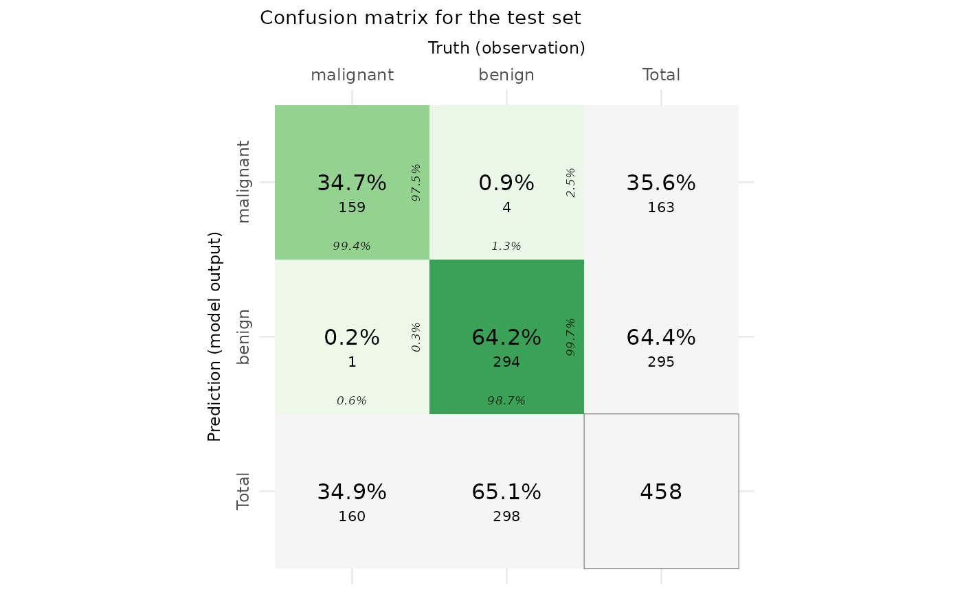
##
## $test_set
Decision curve analysis
The provided code chunk employs the eDecisionCurve function to conduct “decision curve analysis” on the test set within the model. For an in-depth understanding of this methodology, interested readers are encouraged to explore the following authoritative references:
Decision Curve Analysis: https://en.wikipedia.org/wiki/Decision_curve_analysis “Decision curve analysis: a novel method for evaluating prediction models” by Andrew J. Vickers and Elia B. Elkin. Link: https://www.ncbi.nlm.nih.gov/pmc/articles/PMC2577036/ These references offer comprehensive insights into the principles and applications of decision curve analysis, providing a solid foundation for further exploration and understanding of the methodology employed in the presented code.
# enhanced decision curve plot
eDecisionCurve(task = maintask,
trained_model = mylrn,
splits = splits,
seed = seed)Model evaluation (multi-metrics and visual inspection of ROC curves)
By running the next code chunk, you will get the following model evaluation metrics and visualizations:
AUC (Area Under the Curve): AUC quantifies the binary classification model’s performance by assessing the area under the ROC curve, which plots sensitivity against 1-specificity across various threshold values. A value of 0.5 suggests random chance performance, while 1 signifies perfect classification.
BACC (Balanced Accuracy): BACC addresses class imbalance by averaging sensitivity and specificity. Ranging from 0 to 1, a score of 0 indicates chance performance, and 1 signifies perfect classification.
MCC (Matthews Correlation Coefficient): MCC evaluates binary classification model quality, considering true positives, true negatives, false positives, and false negatives. Ranging from -1 to 1, -1 represents complete disagreement, 0 implies chance performance, and 1 indicates perfect classification.
BBRIER (Brier Score): BBRIER gauges the accuracy of probabilistic predictions by measuring the mean squared difference between predicted probabilities and true binary outcomes. Values range from 0 to 1, with 0 indicating perfect calibration and 1 indicating poor calibration.
PPV (Positive Predictive Value): PPV, or precision, measures the proportion of true positive predictions out of all positive predictions made by the model.
NPV (Negative Predictive Value): NPV quantifies the proportion of true negative predictions out of all negative predictions made by the model.
Specificity: Specificity calculates the proportion of true negative predictions out of all actual negative cases in a binary classification problem.
Sensitivity: Sensitivity, also known as recall or true positive rate, measures the proportion of true positive predictions out of all actual positive cases in a binary classification problem.
PRAUC (Precision-Recall Area Under the Curve): PRAUC assesses binary classification model performance based on precision and recall, quantifying the area under the precision-recall curve. A PRAUC value of 1 indicates perfect classification performance.
Additionally, the analysis involves the visualization of ROC and Precision-Recall curves for both development and test sets.
eROC_plot(task = maintask,
trained_model = mylrn,
splits = splits)## [[1]]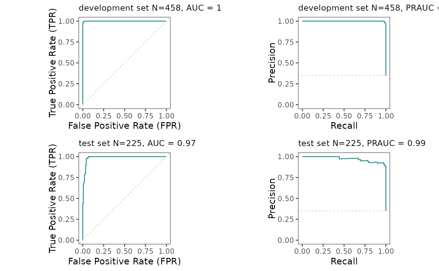
##
## [[2]]
## pred_results$score(measures = mlr3::msrs(meas))
## auc 1.00
## bacc 0.99
## mcc 0.98
## bbrier 0.01
## ppv 0.98
## npv 1.00
## specificity 0.99
## sensitivity 0.99
## prauc 1.00
##
## [[3]]
## pred_results_test$score(measures = mlr3::msrs(meas))
## auc 0.99
## bacc 0.97
## mcc 0.92
## bbrier 0.04
## ppv 0.93
## npv 0.99
## specificity 0.96
## sensitivity 0.97
## prauc 0.97ROC curves with annotated thresholds
By running the next code chunk, you will get ROC and Precision Recall curves for the development and test sets this time with probability threshold information.
ePerformance(task = maintask,
trained_model = mylrn,
splits = splits)## [[1]]
##
## [[2]]
##
## [[3]]loading SHAP results for downstream analysis
Now we can get the outputs from eSHAP_plot function to apply clustering on SHAP values
shap_Mean_wide <- SHAP_output[[2]]
shap_Mean_long <- SHAP_output[[3]]
shap <- SHAP_output[[4]]SHAP values in association with feature values
ShapFeaturePlot(shap_Mean_long)partial dependence of features
Partial dependence plots (PDPs): PDPs can be used to visualize the marginal effect of a single feature on the model prediction.
ShapPartialPlot(shap_Mean_long = shap_Mean_long)extract feature values and predicted probabilities as output of the model to analyze
fval_predprob <- reshape2::dcast(shap, sample_num + pred_prob + predcorrectness ~ feature, value.var = "feature.value")Run a Shiny app to visualize 2-way partial dependence plots
library(shiny)
library(ggplot2)
# assuming your data.table is named `fval_predprob`
ui <- fluidPage(
titlePanel("Feature Plot"),
sidebarLayout(
sidebarPanel(
selectInput("x_feature", "X-axis Feature:",
choices = names(fval_predprob)),
selectInput("y_feature", "Y-axis Feature:",
choices = names(fval_predprob)),
width = 2,
actionButton("stop_button", "Stop")
),
mainPanel(
plotOutput("feature_plot")
)
)
)
server <- function(input, output) {
# create a reactive value for the app state
app_state <- reactiveValues(running = TRUE)
output$feature_plot <- renderPlot({
ggplot(fval_predprob, aes(x = .data[[input$x_feature]], y = .data[[input$y_feature]], fill = pred_prob)) +
geom_tile() +
scale_fill_gradient(low = "white", high = "steelblue", limits = c(0, 1)) +
xlab(input$x_feature) +
ylab(input$y_feature) +
labs(shape = "correct prediction") +
egg::theme_article()
})
# observe the stop button
observeEvent(input$stop_button, {
app_state$running <- FALSE
})
# stop the app if the running state is FALSE
observe({
if(!app_state$running) {
stopApp()
}
})
}
shinyApp(ui = ui, server = server)
str(shap_Mean_long)## tibble [1,980 x 9] (S3: tbl_df/tbl/data.frame)
## $ feature : chr [1:1980] "Bare.nuclei" "Bare.nuclei" "Bare.nuclei" "Bare.nuclei" ...
## $ mean_phi : num [1:1980] 0.0934 0.0934 0.0934 0.0934 0.0934 ...
## $ Phi : num [1:1980] -0.0859 -0.0821 -0.0317 0.0997 0.0817 ...
## $ f_val : num [1:1980] 0 0.111 0 0.444 0.556 ...
## $ unscaled_f_val : num [1:1980] 1 2 1 5 6 1 1 3 1 1 ...
## $ sample_num : int [1:1980] 1 2 3 4 5 6 7 8 9 10 ...
## $ correct_prediction: Factor w/ 2 levels "Incorrect","Correct": 2 2 2 1 2 2 2 2 2 2 ...
## $ pred_prob : num [1:1980] 0.00255 0.00182 0 0.92977 0.9283 ...
## $ pred_class : Factor w/ 2 levels "malignant","benign": 2 2 2 1 1 2 2 1 2 2 ...
# This is the data table that includes SHAP values in wide format. Each row contains sample_num as sample ID and the SHAP values for each feature.
shap_Mean_wide## Key: <sample_num>
## sample_num Bare.nuclei Bl.cromatin Cell.shape Cell.size Cl.thickness
## <int> <num> <num> <num> <num> <num>
## 1: 1 -0.08589487 -0.069985767 -0.04592299 -0.05557913 -0.016991720
## 2: 2 -0.08207815 -0.043686534 -0.06930323 -0.07851767 -0.040950132
## 3: 3 -0.03167399 -0.041501508 -0.05516873 -0.07578722 -0.026012011
## 4: 4 0.09965638 0.100056508 0.16292108 0.13855823 -0.003343413
## 5: 5 0.08170963 0.061670635 0.09991013 0.11153302 -0.024341667
## ---
## 176: 176 -0.10101344 -0.022493651 -0.09723053 -0.11001489 -0.036337381
## 177: 177 -0.07544257 -0.050335159 -0.07331122 -0.07960852 -0.052942063
## 178: 178 -0.07287780 -0.023547804 -0.08396833 -0.07580437 -0.065089868
## 179: 179 -0.12122407 0.054544259 -0.06030249 -0.03421050 -0.088212037
## 180: 180 0.17650148 0.008577434 0.08656048 0.09603124 0.118961111
## Epith.c.size Marg.adhesion Mitoses Normal.nucleoli age
## <num> <num> <num> <num> <num>
## 1: -0.027082751 0.002213201 -0.0022784127 -0.028862540 -0.0037774339
## 2: -0.010480000 -0.018519815 -0.0023586243 -0.016425476 -0.0006488360
## 3: -0.024506111 -0.020070503 -0.0010957672 -0.015432884 -0.0008956349
## 4: 0.076623836 0.041688201 -0.0006521693 0.017386984 0.0067640741
## 5: 0.038122116 0.030285079 0.0018288624 0.029264021 -0.0230379101
## ---
## 176: -0.029844048 -0.031585979 0.0005687831 -0.027441481 -0.0015749206
## 177: -0.024546667 -0.022700053 -0.0008221164 -0.020056270 -0.0021401058
## 178: -0.020292487 -0.024337857 -0.0018688889 -0.019011217 0.0006503175
## 179: -0.030457143 -0.004646905 -0.0040282540 -0.008570794 0.0014429101
## 180: -0.006486825 0.047554444 0.0024593386 0.034816376 -0.0157181481
## sex
## <num>
## 1: 0.0003026190
## 2: -0.0004190476
## 3: 0.0015755556
## 4: 0.0008892857
## 5: 0.0014779101
## ---
## 176: 0.0011694974
## 177: -0.0014722487
## 178: 0.0008101587
## 179: -0.0010852910
## 180: -0.0008616667
# This is the data table of SHAP values in long format and includes feature name, mean_phi_test: mean shap value for the feature across samples, scaled feature values, shap values for each feature, sample ID, and whether the prediction was correct (i.e. predicted class = actual class)
shap_Mean_long## # A tibble: 1,980 x 9
## feature mean_phi Phi f_val unscaled_f_val sample_num correct_prediction
## <chr> <dbl> <dbl> <dbl> <dbl> <int> <fct>
## 1 Bare.nu~ 0.0934 -0.0859 0 1 1 Correct
## 2 Bare.nu~ 0.0934 -0.0821 0.111 2 2 Correct
## 3 Bare.nu~ 0.0934 -0.0317 0 1 3 Correct
## 4 Bare.nu~ 0.0934 0.0997 0.444 5 4 Incorrect
## 5 Bare.nu~ 0.0934 0.0817 0.556 6 5 Correct
## 6 Bare.nu~ 0.0934 -0.0518 0 1 6 Correct
## 7 Bare.nu~ 0.0934 -0.113 0 1 7 Correct
## 8 Bare.nu~ 0.0934 -0.00175 0.222 3 8 Correct
## 9 Bare.nu~ 0.0934 -0.0468 0 1 9 Correct
## 10 Bare.nu~ 0.0934 -0.221 0 1 10 Correct
## # i 1,970 more rows
## # i 2 more variables: pred_prob <dbl>, pred_class <fct>Patient subgroups determined by SHAP clusters
SHAP clustering is a method to better understand why a model may perform better for some patients than others. Here for example, you can identify patient subgroups that have specific patterns that are different from other subgroups and that explains why the model you developed have perhaps better or worse performance for those patients than the average performance for the whole dataset. You can see the difference in the SHAP plots that if you group all together provide the overall SHAP summary plot. Again here the edges reflect how features may interact with each other in each individual sample (instance).
# the number of clusters can be changed
SHAP_plot_clusters <- SHAPclust(task = maintask,
trained_model = mylrn,
splits = splits,
shap_Mean_wide = shap_Mean_wide,
shap_Mean_long = shap_Mean_long,
num_of_clusters = 3,
seed = seed,
subset = .8)## Key: <sample_num, feature, Phi>
## sample_num feature Phi cluster mean_phi f_val
## <int> <char> <num> <int> <num> <num>
## 1: 1 Bare.nuclei -0.0858948677 3 0.093444244 0.0000000
## 2: 1 Bl.cromatin -0.0699857672 3 0.044548987 0.0000000
## 3: 1 Cell.shape -0.0459229894 3 0.076720237 0.0000000
## 4: 1 Cell.size -0.0555791270 3 0.091198097 0.0000000
## 5: 1 Cl.thickness -0.0169917196 3 0.069835393 0.5000000
## ---
## 1976: 180 Marg.adhesion 0.0475544444 2 0.026453762 1.0000000
## 1977: 180 Mitoses 0.0024593386 2 0.002165296 0.1250000
## 1978: 180 Normal.nucleoli 0.0348163757 2 0.021391343 0.7777778
## 1979: 180 age -0.0157181481 2 0.003230698 0.0000000
## 1980: 180 sex -0.0008616667 2 0.001183048 0.0000000
## unscaled_f_val correct_prediction pred_prob pred_class
## <num> <fctr> <num> <fctr>
## 1: 1 Correct 0.002554762 benign
## 2: 1 Correct 0.002554762 benign
## 3: 1 Correct 0.002554762 benign
## 4: 1 Correct 0.002554762 benign
## 5: 5 Correct 0.002554762 benign
## ---
## 1976: 10 Correct 0.926616667 malignant
## 1977: 2 Correct 0.926616667 malignant
## 1978: 8 Correct 0.926616667 malignant
## 1979: 18 Correct 0.926616667 malignant
## 1980: 1 Correct 0.926616667 malignant## Warning in geom_jitter(aes(shape = correct_prediction, text = paste("Feature:
## ", : Ignoring unknown aesthetics: text## Warning in check_gg_image_packages(add_arrows = add_arrows, add_zero_shading =
## add_zero_shading): 'ggimage' is missing. Will not plot arrows and zero-shading.## Warning in check_gg_image_packages(add_arrows = add_arrows, add_zero_shading =
## add_zero_shading): 'rsvg' is missing. Will not plot arrows and zero-shading.## Warning in check_gg_image_packages(add_arrows = add_arrows, add_zero_shading =
## add_zero_shading): 'ggimage' is missing. Will not plot arrows and zero-shading.## Warning in check_gg_image_packages(add_arrows = add_arrows, add_zero_shading =
## add_zero_shading): 'rsvg' is missing. Will not plot arrows and zero-shading.
# note that the subset must be the same value as the SHAP analysis done earlier
# display the SHAP cluster plots
SHAP_plot_clusters[[1]]
# display the confusion matrices corresponding to the SHAP clusters (patient subsets determined by SHAP clusters)
SHAP_plot_clusters[[2]]
Model fairness (sensitivity analysis)
Sometimes we would like to investigate whether our model performs fairly well for different subgroups based on categories of variables such as sex.
# you should decide what variables to use to be tested
# here we chose sex from the variables existing in the dataset
Fairness_results <- eFairness(task = maintask,
trained_model = mylrn,
splits = splits,
target_variable = "sex",
var_levels = c("Male", "Female"))## Warning in verify_d(data$d): D not labeled 0/1, assuming benign = 0 and
## malignant = 1!
## Warning in verify_d(data$d): D not labeled 0/1, assuming benign = 0 and
## malignant = 1!
## Warning in verify_d(data$d): D not labeled 0/1, assuming benign = 0 and
## malignant = 1!
# ROC curves for the subgroups for the development (left) and test (right) sets
Fairness_results[[1]]
# performance in the subgroups for the development set
Fairness_results[[2]]## Male Female
## auc 1.00 1.00
## bacc 0.99 0.99
## mcc 0.97 0.98
## bbrier 0.01 0.01
## ppv 0.96 0.99
## npv 1.00 0.99
## specificity 0.98 0.99
## sensitivity 1.00 0.99
## prauc 1.00 1.00
# performance in the subgroups for the test set
Fairness_results[[3]]## Male Female
## auc 0.98 0.99
## bacc 0.98 0.96
## mcc 0.94 0.91
## bbrier 0.04 0.03
## ppv 0.92 0.93
## npv 1.00 0.97
## specificity 0.96 0.96
## sensitivity 1.00 0.95
## prauc 0.96 0.98Model parameters
# get model parameters
model_params <- mylrn$param_set
print(data.table::as.data.table(model_params))## id class lower upper
## <char> <char> <num> <num>
## 1: always.split.variables ParamUty NA NA
## 2: class.weights ParamUty NA NA
## 3: holdout ParamLgl NA NA
## 4: importance ParamFct NA NA
## 5: keep.inbag ParamLgl NA NA
## 6: max.depth ParamInt 1 Inf
## 7: min.bucket ParamUty NA NA
## 8: min.node.size ParamUty NA NA
## 9: mtry ParamInt 1 Inf
## 10: mtry.ratio ParamDbl 0 1
## 11: na.action ParamFct NA NA
## 12: num.random.splits ParamInt 1 Inf
## 13: node.stats ParamLgl NA NA
## 14: num.threads ParamInt 1 Inf
## 15: num.trees ParamInt 1 Inf
## 16: oob.error ParamLgl NA NA
## 17: regularization.factor ParamUty NA NA
## 18: regularization.usedepth ParamLgl NA NA
## 19: replace ParamLgl NA NA
## 20: respect.unordered.factors ParamFct NA NA
## 21: sample.fraction ParamDbl 0 1
## 22: save.memory ParamLgl NA NA
## 23: scale.permutation.importance ParamLgl NA NA
## 24: seed ParamInt -Inf Inf
## 25: split.select.weights ParamUty NA NA
## 26: splitrule ParamFct NA NA
## 27: verbose ParamLgl NA NA
## 28: write.forest ParamLgl NA NA
## id class lower upper
## levels nlevels is_bounded
## <list> <num> <lgcl>
## 1: [NULL] Inf FALSE
## 2: [NULL] Inf FALSE
## 3: TRUE,FALSE 2 TRUE
## 4: none,impurity,impurity_corrected,permutation 4 TRUE
## 5: TRUE,FALSE 2 TRUE
## 6: [NULL] Inf FALSE
## 7: [NULL] Inf FALSE
## 8: [NULL] Inf FALSE
## 9: [NULL] Inf FALSE
## 10: [NULL] Inf TRUE
## 11: na.learn,na.omit,na.fail 3 TRUE
## 12: [NULL] Inf FALSE
## 13: TRUE,FALSE 2 TRUE
## 14: [NULL] Inf FALSE
## 15: [NULL] Inf FALSE
## 16: TRUE,FALSE 2 TRUE
## 17: [NULL] Inf FALSE
## 18: TRUE,FALSE 2 TRUE
## 19: TRUE,FALSE 2 TRUE
## 20: ignore,order,partition 3 TRUE
## 21: [NULL] Inf TRUE
## 22: TRUE,FALSE 2 TRUE
## 23: TRUE,FALSE 2 TRUE
## 24: [NULL] Inf FALSE
## 25: [NULL] Inf FALSE
## 26: gini,extratrees,hellinger 3 TRUE
## 27: TRUE,FALSE 2 TRUE
## 28: TRUE,FALSE 2 TRUE
## levels nlevels is_bounded
## special_vals default storage_type tags
## <list> <list> <char> <list>
## 1: <list[0]> <NoDefault[0]> list train
## 2: <list[0]> [NULL] list train
## 3: <list[0]> FALSE logical train
## 4: <list[0]> <NoDefault[0]> character train
## 5: <list[0]> FALSE logical train
## 6: <list[1]> [NULL] integer train
## 7: <list[0]> 1 list train
## 8: <list[1]> [NULL] list train
## 9: <list[1]> <NoDefault[0]> integer train
## 10: <list[0]> <NoDefault[0]> numeric train
## 11: <list[0]> na.learn character train
## 12: <list[0]> 1 integer train
## 13: <list[0]> FALSE logical train
## 14: <list[0]> 1 integer train,predict,threads
## 15: <list[0]> 500 integer train,predict,hotstart
## 16: <list[0]> TRUE logical train
## 17: <list[0]> 1 list train
## 18: <list[0]> FALSE logical train
## 19: <list[0]> TRUE logical train
## 20: <list[0]> <NoDefault[0]> character train
## 21: <list[0]> <NoDefault[0]> numeric train
## 22: <list[0]> FALSE logical train
## 23: <list[0]> FALSE logical train
## 24: <list[1]> [NULL] integer train,predict
## 25: <list[0]> [NULL] list train
## 26: <list[0]> gini character train
## 27: <list[0]> TRUE logical train,predict
## 28: <list[0]> TRUE logical train
## special_vals default storage_type tags