SHAP analysis in multi-class classification tasks

Load Required Libraries

We will begin by loading the necessary packages.

library(explainer)
library(mlbench)
library(mlr3learners)

## Loading required package: mlr3

library(ranger)
library(iml)
library(dplyr)

## 
## Attaching package: 'dplyr'

## The following objects are masked from 'package:stats':
## 
##     filter, lag

## The following objects are masked from 'package:base':
## 
##     intersect, setdiff, setequal, union

library(ggplot2)
library(plotly)

## 
## Attaching package: 'plotly'

## The following object is masked from 'package:ggplot2':
## 
##     last_plot

## The following object is masked from 'package:stats':
## 
##     filter

## The following object is masked from 'package:graphics':
## 
##     layout

library(cvms)
library(ggplot2)
library(gridExtra)

## 
## Attaching package: 'gridExtra'

## The following object is masked from 'package:dplyr':
## 
##     combine

Set Seed for Reproducibility

seed <- 246
set.seed(seed)

Load and Prepare the Data

We will use the Iris dataset for this example and define the target column (Species).

# Load the Iris dataset
data("iris")
target_col <- "Species"

# Extract relevant columns from the dataset
mydata <- iris

Create the Classification Task

We create a classification task using the mlr3 package.

maintask <- mlr3::TaskClassif$new(
  id = "my_classification_task",
  backend = mydata,
  target = target_col
)

Split the Dataset

We will split the data into training and test sets.

splits <- mlr3::partition(maintask, ratio = 0.3)

Train the Model

Using the ranger algorithm, we will train a classification model.

mylrn <- mlr3::lrn("classif.ranger", predict_type = "prob")
mylrn$train(maintask, splits$train)

Make Predictions

Once the model is trained, we make predictions on the test set.

# Make predictions on the test set
predictions <- mylrn$predict(maintask, splits$test)

# Convert predictions to a data frame
predicted_classes <- predictions$response
true_classes <- mydata[splits$test, target_col]

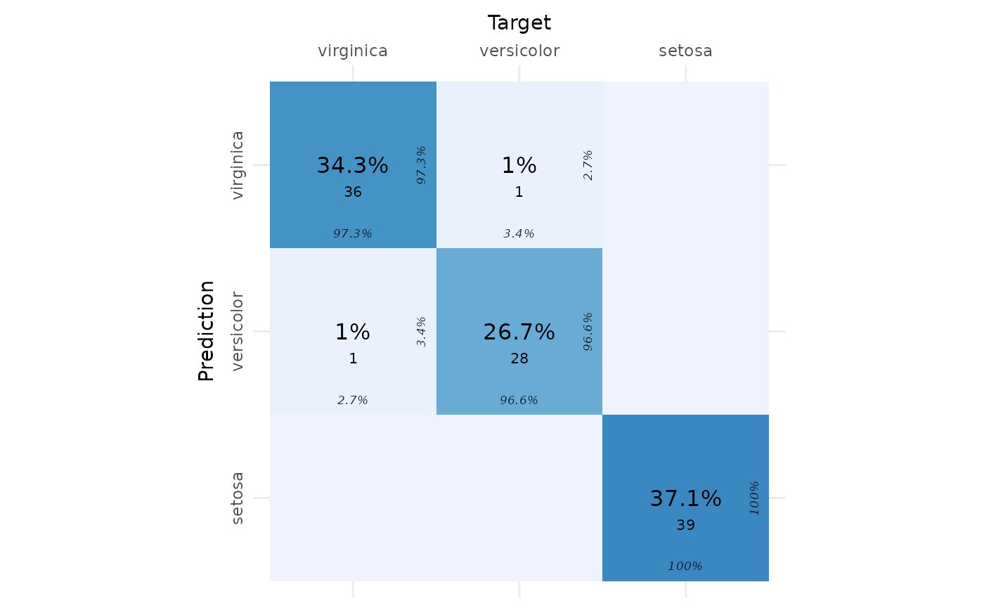
Confusion Matrix

We create and visualize a confusion matrix using the cvms package.

# Create a confusion matrix
conf_matrix <- table(True = true_classes, Predicted = predicted_classes)

# Convert the confusion matrix to a data frame with required column names
conf_matrix_df <- as.data.frame(conf_matrix)
colnames(conf_matrix_df) <- c("Target", "Prediction", "N")

# Plot the confusion matrix
plot_confusion_matrix(conf_matrix_df)

## Warning in plot_confusion_matrix(conf_matrix_df): 'ggimage' is missing. Will
## not plot arrows and zero-shading.

## Warning in plot_confusion_matrix(conf_matrix_df): 'rsvg' is missing. Will not
## plot arrows and zero-shading.

SHAP (SHapley Additive exPlanations) Analysis

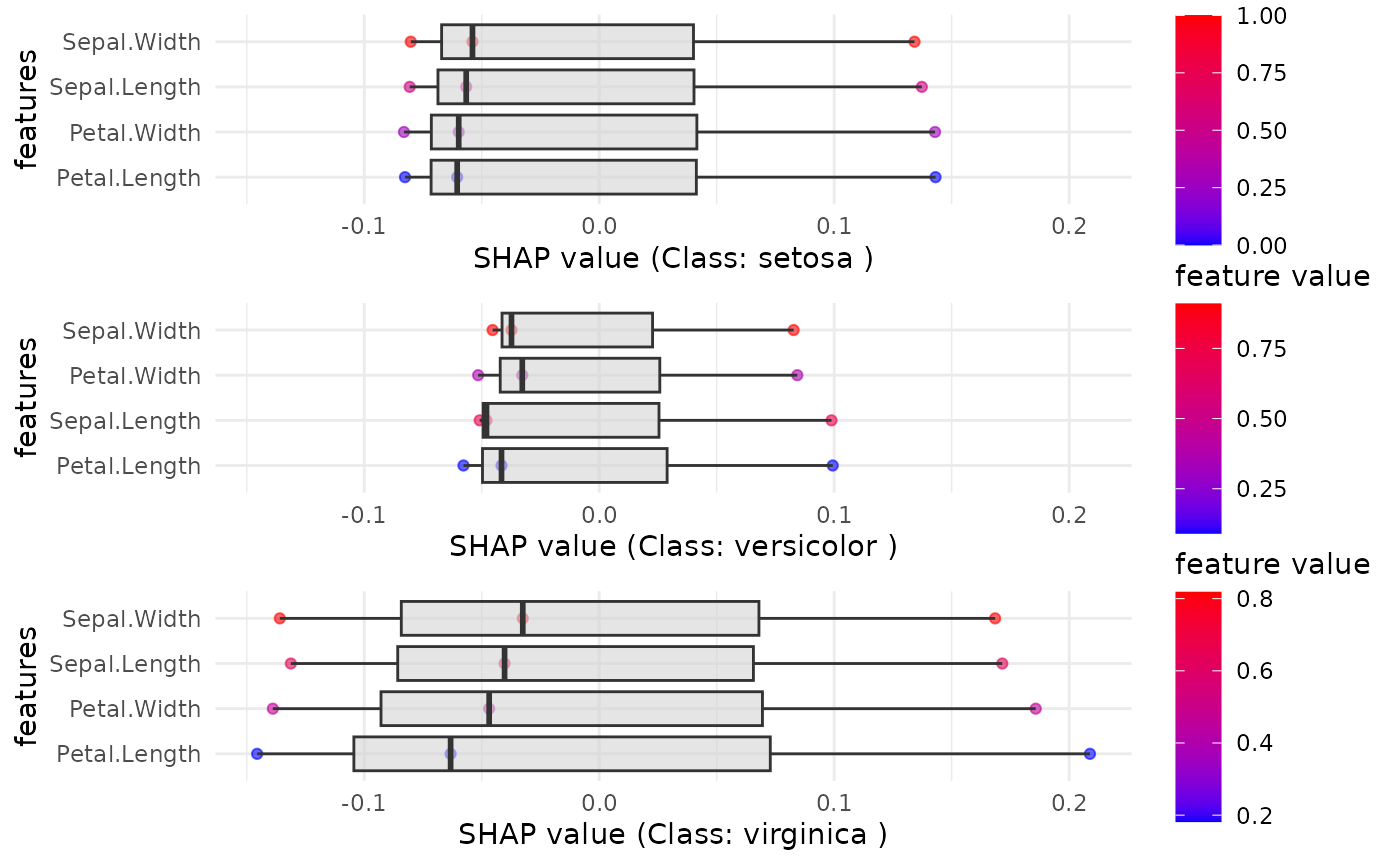
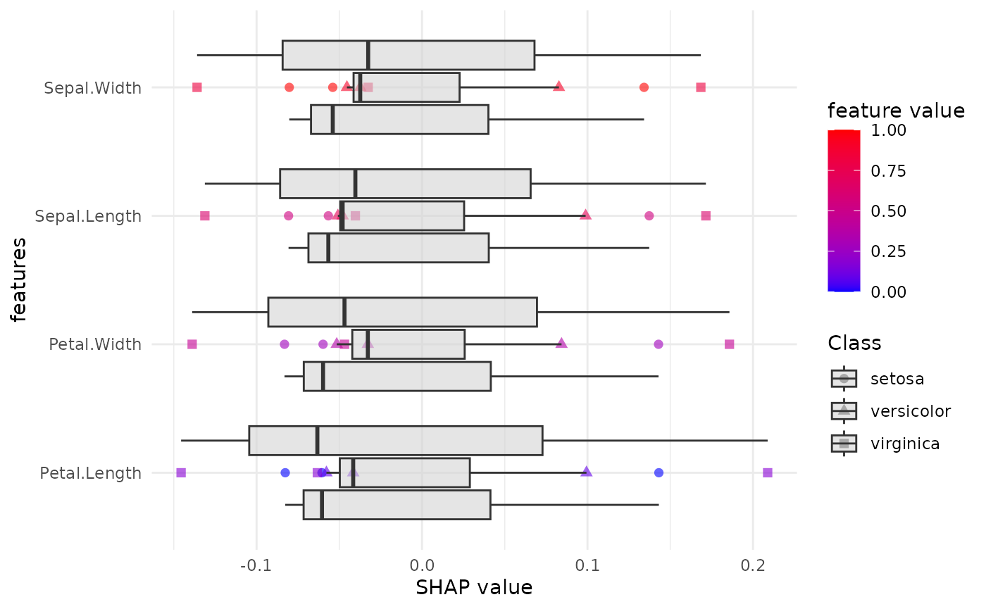
We will now compute SHAP values for the dataset to understand the feature importance for each class.

We now use the SHAP function to generate the SHAP plots for each class and a combined plot for all classes.

SHAP_output <- eSHAP_plot_multiclass(
  task = maintask,
  trained_model = mylrn,
  splits = splits,
  sample.size = 30,
  seed = seed,
  subset = 0.8
)

# Display the combined SHAP plot for each class
print(SHAP_output$combined_plot)

## TableGrob (3 x 1) "arrange": 3 grobs
##            z     cells    name           grob
## setosa     1 (1-1,1-1) arrange gtable[layout]
## versicolor 2 (2-2,1-1) arrange gtable[layout]
## virginica  3 (3-3,1-1) arrange gtable[layout]

Display the combined plot for all classes together

print(SHAP_output$combined_all_classes)

Notes:

This script loads the Iris dataset, trains a classifier using the ranger algorithm, makes predictions, creates a confusion matrix, and calculates SHAP values for feature importance.
SHAP values are visualized per class and across all classes using ggplot2.

Ramtin Zargari Marandi